Cleaning Data
For my CSUCI lab group I cleaned messy data with many missing values, I also programmatically added a day/night column using a REST API.
The raw data was loaded from temperature probes ‘IBUTTONs’ fixed in inter tidal regions on Santa Rosa Island, CA. There are two locations on the island where probes are installed, Beachers Bay ‘BB’ and Skunk Point ‘SP’. At each of these two locations IBUTTONs are situated at 4 different tidal zones: Low ‘L’, Mid ‘M’, High ‘H’, and Splash ‘S’. For each of these tidal levels there are 5 IBUTTONs. BB-L1, BB-L2, BB-L3, etc.
When this data was originally cleaned and mutated the previous researcher added information to indicate if the IBUTTON was out of water ‘OOW’ by using tide height. The researcher also added a column to indicate day or night, which appears to be inaccurate
Packages Used
library(readr); library(readxl); library(stringr)
library(chron); library(ggplot2); library(tibble);
library(dplyr); library(tidyr); library(visdat);
library(httr); library(jsonlite); library(magrittr)
Parsing Excel Data
The Excel file ‘IBUTTON_MASTER_DATA.xlsx’ contains two sheets ‘BB’ and ‘SP’
pathToXLSX <- "/Users/smcatee/Desktop/TF/IBUTTON/IBUTTON_MASTER_DATA.xlsx"
readxl::excel_sheets(path = pathToXLSX)
## [1] "SP" "BB"# Load each sheet
masterData_SP <- readxl::read_xlsx(path = pathToXLSX, sheet = "SP", na = c("", "NA", "NaN"))
masterData_BB <- readxl::read_xlsx(path = pathToXLSX, sheet = "BB", na = c("", "NA", "NaN"))Both BB and SP tables have similar sizes.
dim(masterData_SP)
dim(masterData_BB)
## [1] 25388 224
## [1] 25392 225The column names are also similar for both tables.
tibble::tibble(
  "BB_ColNames" = masterData_BB %>% colnames() %>% head(10),
  "SP_ColNames" = masterData_SP %>% colnames() %>% head(10)
  )
## # A tibble: 10 x 2
## BB_ColNames SP_ColNames
## <chr> <chr>
## 1 DATE TIME date
## 2 date time
## 3 time tide offset
## 4 tide offset tide height transformed
## 5 tide height transformed L1
## 6 L1 Temp L1 Height
## 7 L1 Height l1 height tranformed
## 8 l1 height tranformed L1-TideHeight
## 9 L1-TideHeight L1 OOW? [TRUE/FALSE]
## 10 L1 OOW? [TRUE/FALSE] SunRise...10Not all of the these columns need to be kept since some were intermediate steps made by the previous researcher.
The only important columns are the date/time, temperature, and OOW (Out Of Water). There are columns date, time, and DATE TIME. This is a bit confusing so lets explore their values…
tibble::tibble(
  "DATE_TIME" = masterData_BB$`DATE TIME` %>% head(),
  "date" = masterData_BB$date %>% head(),
  "time" = masterData_BB$time %>% head()
)
## # A tibble: 6 x 3
## DATE_TIME date time
## <dbl> <dttm> <time>
## 1 NaN 2016-03-31 00:00:00 23:33
## 2 NaN 2016-04-01 00:00:00 00:33
## 3 NaN 2016-04-01 00:00:00 01:33
## 4 NaN 2016-04-01 00:00:00 02:33
## 5 NaN 2016-04-01 00:00:00 03:33
## 6 NaN 2016-04-01 00:00:00 04:33It looks like DATE TIME might have been an Excel formula that was corrupted. The date column and the time column appear to be real dates and times from the IBUTTON readings.
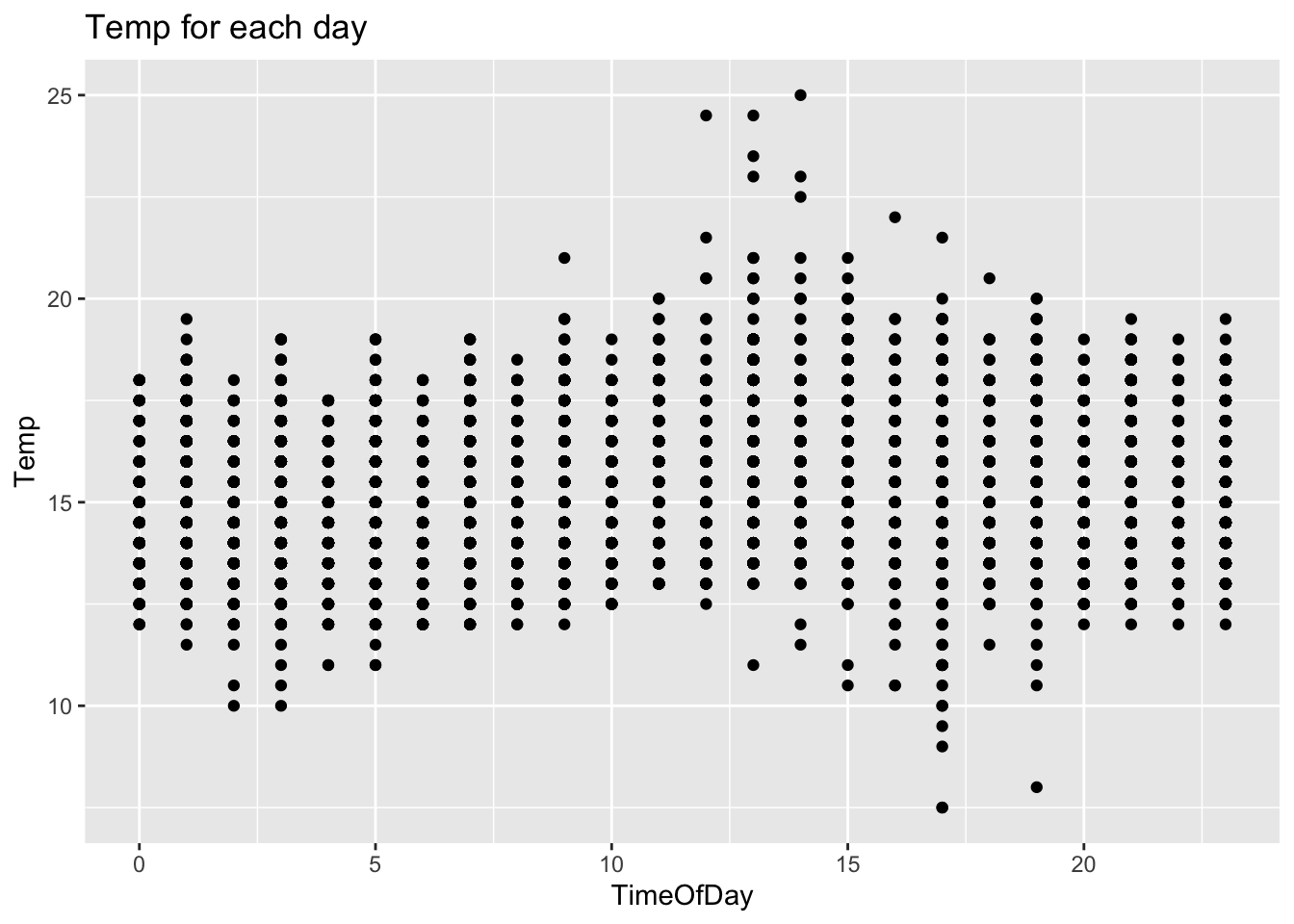
For a quick sanity check, a plot can be made to show the temperature fluctuating through a 24 hour period.
masterData_BB %>%
  select(3, 6) %>%
  transmute(timeOfDay = hours(as.times(time)), Temp = as.numeric(`L1 Temp`)) %>%
  ggplot(aes(timeOfDay, Temp)) +
    geom_point() +
    labs(title = "Temp for each day", x = "TimeOfDay", y = "Temp")
In general the temperature peak appears to be at 13:00 and the trough appears to be at 03:00. Looks good, lets move on..
Data Selection
Now we have a distinct list of columns to keep:
- Date = date
- Time = time
- Temperature = L1 Temp, L1, L2 Temp, L2, …
- OOW = L1 OOW?, L2 OOW?, …
It would be easy enough to select columns by hand, but here is some automation for practice
regexPattern <- "(^date$)|(^time$)|(^[LMHS][1-5]( [Tt]emp)?$)|(OOW\\?)"
ibutton_SP <- masterData_SP %>%
  dplyr::select(matches(match = regexPattern, ignore.case = FALSE))
ibutton_BB <- masterData_BB %>%
  dplyr::select(matches(match = regexPattern, ignore.case = FALSE))
# Sanity check
ibutton_SP %>% colnames() %>% head()
ibutton_BB %>% colnames() %>% head()## [1] "date" "time" "L1"
## [4] "L1 OOW? [TRUE/FALSE]" "L2" "L2 OOW? [TRUE/FALSE]"
## [1] "date" "time" "L1 Temp"
## [4] "L1 OOW? [TRUE/FALSE]" "L2 Temp" "L2 OOW? [TRUE/FALSE]"The column names are odd, so here are better names
newColNames <- colnames(ibutton_SP)
newColNames[1] <- "Date"
newColNames[2] <- "Time"
newColNames %<>% str_replace(fixed(" Temp"), "_Temperature")
newColNames %<>% sapply(
                  function(colName){
                    if_else(
                      str_detect(colName, "^..$"),
                      paste0(colName, "_Temperature"),
                      colName)
                    },
                  USE.NAMES = FALSE
                  )

newColNames %<>% str_replace(" OOW.*", "_isSubmerged")
colnames(ibutton_SP) <- newColNames
colnames(ibutton_BB) <- newColNames
# Sanity check
colnames(ibutton_SP) %>% head()## [1] "Date" "Time" "L1_Temperature" "L1_isSubmerged"
## [5] "L2_Temperature" "L2_isSubmerged"colnames(ibutton_BB) %>% head()## [1] "Date" "Time" "L1_Temperature" "L1_isSubmerged"
## [5] "L2_Temperature" "L2_isSubmerged"
Visualize value types
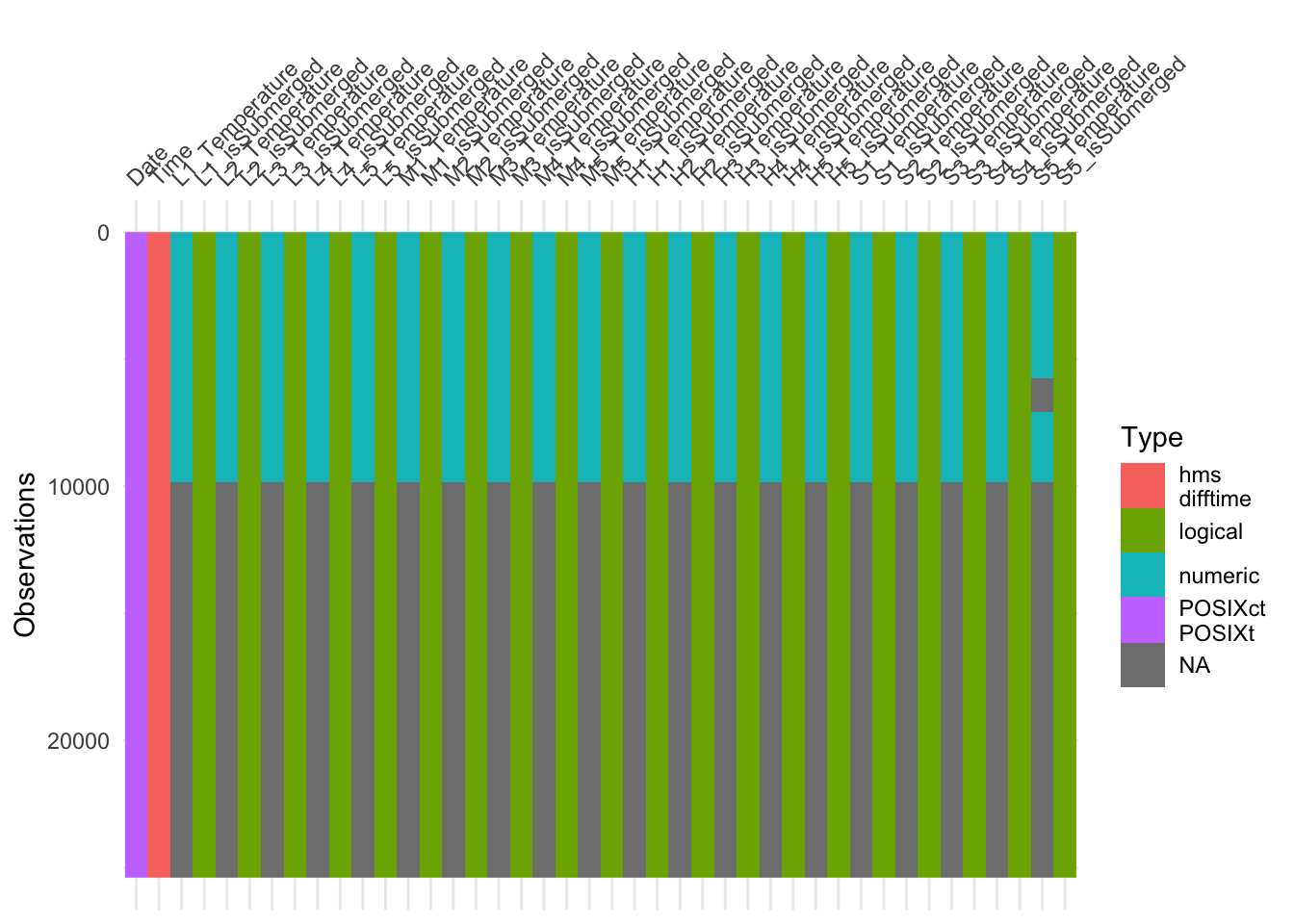
The handy package visdat can be used to plot value types for whole tables.
visdat::vis_dat(ibutton_SP, sort_type = FALSE, warn_large_data = FALSE)
The whole bottom half of ibutton_SP is missing! This is handled easily below.
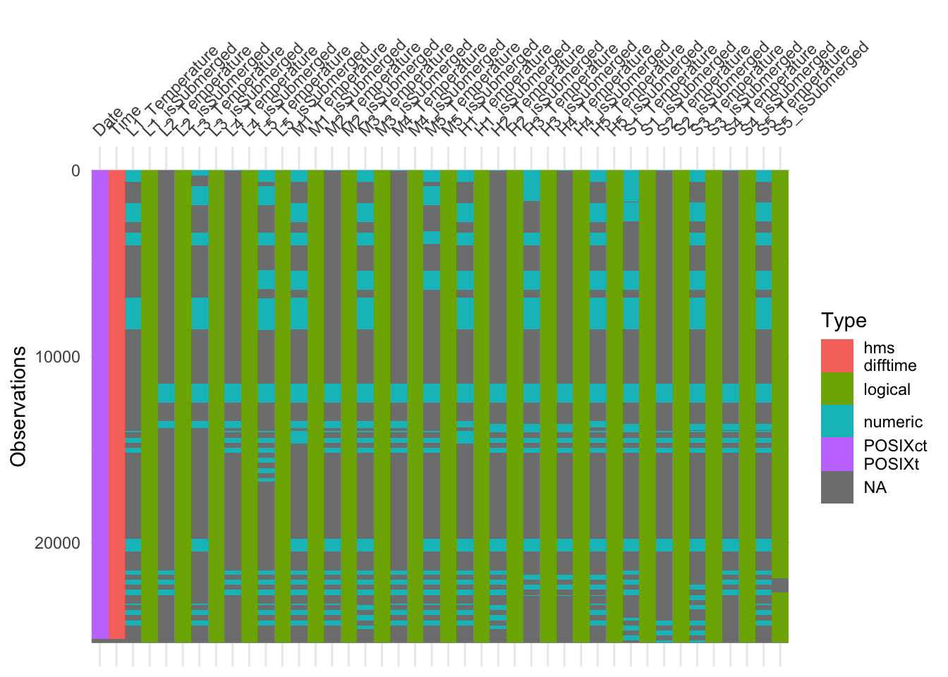
Lets check ibutton_BB.
visdat::vis_dat(ibutton_BB, sort_type = FALSE, warn_large_data = FALSE)
Intermittent data is missing in ibutton_BB. This missing data can be handled in a few more steps. The consequences of the missing data for both tables will have to be considered during the data analysis stage.
Here, ibutton_SP missing values can be removed by only selecing rows with non-NA values in any column, except for S5_Temperature
ibutton_SP <- ibutton_SP[!is.na(ibutton_SP$L1_Temperature),]Here, ibutton_BB missing values can not be removed by taking out whole rows since some rows are full of NA values while other rows still have some non-NA values. The first step will be selecting the indexes for Temperature columns, the second step will be selecting temperature rows that have some non-NA values, then the third step will be selecting Date and Time rows that have non-NA values.
temperatureColIndexes <- ibutton_BB %>% colnames() %>% str_detect("_Temperature") %>% which()

temp_nonNA_rows <- ibutton_BB[temperatureColIndexes] %>% is.na() %>%
  rowSums() != length(temperatureColIndexes)

dateTime_nonNA_rows <- ibutton_BB[c(1,2)] %>% is.na() %>% rowSums() != 2

ibutton_BB <- ibutton_BB[temp_nonNA_rows & dateTime_nonNA_rows,]
Now both tables will have rows with non-NA Date and Time and at least one non-NA temperature value.
visdat::vis_dat(ibutton_SP, sort_type = FALSE, warn_large_data = FALSE)
visdat::vis_dat(ibutton_BB, sort_type = FALSE, warn_large_data = FALSE)
Creating isDay column
Now that the tables are cleaned the final step is to create an isDay column that will use sunrise/sunset data that can be called from ‘api.sunrise-sunset.org’
for (step in c(1,2)) {
  if(step == 1) {curTable <- ibutton_SP}
  if(step == 2) {curTable <- ibutton_BB}

  # Assemble a vector that will become the isDay column
  isDayCol <- c()
  nDays <- 0
  rowIndex <- 1
  while( rowIndex <= nrow(curTable) ) {

    # GET sunrise and sunset times for chunks of rows with the same date
    # using sunrise-sunset.org REST API
    curDate <- as.Date(curTable$Date[rowIndex])
    call <- paste0("https://api.sunrise-sunset.org/json?lat=36.7201600&lng=-4.4203400  &date=", curDate)
    callContent <- httr::content(GET(call), "text")
    callContentJSON <- jsonlite::fromJSON(callContent, flatten=TRUE)
    sunrise <- chron::as.times(stringr::str_remove(callContentJSON$results$sunrise, " AM"))
    sunset <- chron::as.times(stringr::str_remove(callContentJSON$results$sunset, " PM")) + as.times("12:00:00")

    # For chunks of rows with the same date compare sunrise/sunset to time
    while (curDate == as.Date(curTable$Date[rowIndex])) {

      isDay <- FALSE
      curTime <- curTable$Time[rowIndex] %>% as.character()
      isDay <- ifelse(curTime < sunrise | curTime > sunset, FALSE, TRUE)
      isDayCol <- c(isDayCol, isDay)

      rowIndex = rowIndex + 1
      if( rowIndex > nrow(curTable) ) { break }
    }
  }
  curTable <- tibble::add_column(curTable, isDay=isDayCol, .after = "Time")
  curTable %>% colnames()
  curTable$isDay %>% table()

  if(step == 1) {ibutton_SP <- curTable}
  if(step == 2) {ibutton_BB <- curTable}
}
Checking that the isDay column produced only TRUE and FALSE values:
ibutton_SP$isDay %>% table()## .
## FALSE TRUE
## 4751 5072ibutton_BB$isDay %>% table()## .
## FALSE TRUE
## 6868 6866
Tidy up
The data is clean, but is not necessarily ‘tidy’. Following the tidy data principles this table is too ‘wide’ and must be converted to a ‘long’ format. The site names (e.g. L1, M2…) should be values in a column named ‘Site’. The resulting table will have only 6 columns: Date Time isDay Site Temperature isSubmerged
The Temperature and isSubmerged column names both contain the same Site values (e.g. L1, S4, …). It will be easier to lengthen Temperature and isSubmerged columns independently, creating new Site columns for each. Then columns from both lengthened tables can be joined as a new tibble.
# select out isSubmerged columns into separate df
ibutton_SP_subm <- ibutton_SP %>% dplyr::select(ends_with("isSubmerged"))

# pivot_longer temperature table
ibutton_SP_temp <- ibutton_SP %>%
  tidyr::pivot_longer(
    cols = ends_with("Temperature"),
    names_to = c("Site","eraseMe"),
    values_to = "Temperature",
    values_drop_na = FALSE,
    names_sep = "_"
    ) %>%
  dplyr::select(Date, Time, isDay, Site, Temperature)

# pivot_longer isSubmerged table
ibutton_SP_subm <- ibutton_SP_subm %>%
  tidyr::pivot_longer(
    cols = ends_with("isSubmerged"),
    names_to = c("Site", "eraseMe"),
    values_to = "isSubmerged",
    values_drop_na = FALSE,
    names_sep = "_"
  ) %>% dplyr::select(-eraseMe)

# recombine
ibutton_SP <- tibble::add_column(ibutton_SP_temp, isSubmerged = ibutton_SP_subm$isSubmerged, .after = "Temperature")
This chunk is then mirrored for ibutton_BB
Visualizing the tidy data
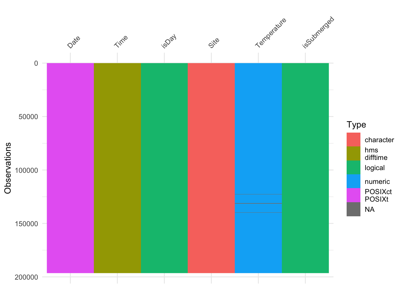
Now that the tables are long they are visually less appealing, but they are far easier to analyze in R.
visdat::vis_dat(ibutton_SP, sort_type = FALSE, warn_large_data = FALSE)
visdat::vis_dat(ibutton_BB, sort_type = FALSE, warn_large_data = FALSE)
ibutton_SP %>% head(10)## # A tibble: 10 x 6
## Date Time isDay Site Temperature isSubmerged
## <dttm> <time> <lgl> <chr> <dbl> <lgl>
## 1 2016-03-31 00:00:00 23:33 FALSE L1 15.3 TRUE
## 2 2016-03-31 00:00:00 23:33 FALSE L2 0 FALSE
## 3 2016-03-31 00:00:00 23:33 FALSE L3 14.5 FALSE
## 4 2016-03-31 00:00:00 23:33 FALSE L4 0 FALSE
## 5 2016-03-31 00:00:00 23:33 FALSE L5 15 FALSE
## 6 2016-03-31 00:00:00 23:33 FALSE M1 16.3 TRUE
## 7 2016-03-31 00:00:00 23:33 FALSE M2 0 TRUE
## 8 2016-03-31 00:00:00 23:33 FALSE M3 16.3 TRUE
## 9 2016-03-31 00:00:00 23:33 FALSE M4 0 TRUE
## 10 2016-03-31 00:00:00 23:33 FALSE M5 15.7 FALSEibutton_BB %>% head(10)## # A tibble: 10 x 6
## Date Time isDay Site Temperature isSubmerged
## <dttm> <time> <lgl> <chr> <dbl> <lgl>
## 1 2016-03-31 00:00:00 23:33 FALSE L1 14.5 FALSE
## 2 2016-03-31 00:00:00 23:33 FALSE L2 NaN FALSE
## 3 2016-03-31 00:00:00 23:33 FALSE L3 14.5 FALSE
## 4 2016-03-31 00:00:00 23:33 FALSE L4 0 FALSE
## 5 2016-03-31 00:00:00 23:33 FALSE L5 14.5 FALSE
## 6 2016-03-31 00:00:00 23:33 FALSE M1 14.5 TRUE
## 7 2016-03-31 00:00:00 23:33 FALSE M2 0 TRUE
## 8 2016-03-31 00:00:00 23:33 FALSE M3 14 TRUE
## 9 2016-03-31 00:00:00 23:33 FALSE M4 0 TRUE
## 10 2016-03-31 00:00:00 23:33 FALSE M5 14.5 TRUESave the output!
write_csv(ibutton_SP, "/Users/smcatee/Desktop/TF/IBUTTON/IBUTTON_SP.csv")
write_csv(ibutton_BB, "/Users/smcatee/Desktop/TF/IBUTTON/IBUTTON_BB.csv")
Next, check out my example of time series analysis!
